Markowitz Model and Modern Portfolio Theory – Explained [YTNote]

This is a Youtube video Note.

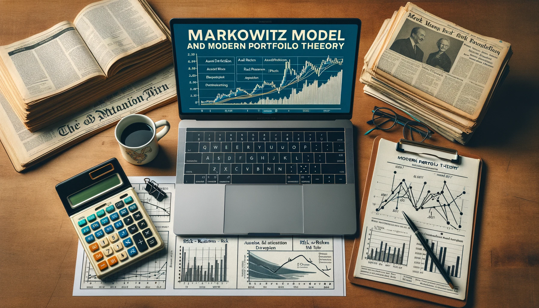
MPT first by Markowitz. Markowitz suggested that the asset’s volatility was a good metric to use to assess total risk. In other words, the more volatile an asset’s price, the more risk this asset posed to an investor. Also the riskier asset has also better possibility of payoff more than the less risky asset.

Markowitz suggested :

• Assets moving correlated and correlated to one another. Therefore some assets would move together in a similar fashion.

So he believes that correlations and covariances between assets were important. He summarized this relationship in a covariance matrix called Sigma. Sigma can simply be thought of as a matrix made up of the time series covariances of each asset.

What Markowitz also considered was that there was an infinite combination of allocations between assets a person could put into their portfolio. However, there was only a subset of combinations that he believed were the efficient allocations. These efficient allocations lived along a curve, which Markowitz called the Efficient Frontier. Allocations which lived along this efficient frontier were considered to have the best reward for a given level of risk.

So how we calculate this curve using our covariance matrix ?

We know that we can have some set of portfolio weights for each of our assets. we will call this portfolio vector of weights as w .

w = [w_1,w_2,w_3,w_4...,w_n]

If we multiply a vector of weights by our covariance matrix by the transpose of our vector weights, we get a volatility^2 term ( or standard deviation ^2 term for the statisticians friends )

We want to know is when is this value minimized for a given level of returns.

We will call this level of Returns, R , and so how do we calculate R ?

But let’s just say for now, that for each of our assets we have calculated has an expected return value we believe is appropriate.

We will put those return values into a new vector called Mu.

\mu = [r_1,r_2,r_3...r_n]

Logically, if we multiply Mu by the transpose of our weights W , then we get a portfolio return of R.

Now we have our two equations:

• Risk equation
• Return equation

and we want to minimize one of them and maximize another one.

In other words, we want to minimize Risk and Maximize returns,

Because these two systems are consistent and underdetermined, we get a curve as our solution.

We can solve for any point on the curve using the equation w equals lambda times the inverse of Sigma times Mu.

Lambda is your risk tolerance and ranges from 0 ( no risk ) to infinity ( unlimited risk ).

The reward of the MPT is that by diversifying your assets that have opposing correlations but positive expected returns, investors can theoretically maximize return and minimize risks.

We mentioned earlier in the video expected returns, so how do we calculate expected returns ?

Calculation of mu is different from person to person and it really is the secret sauce behind a great portfolio investment strategy. One way that many financial experts have used to calculate expected returns is related to some of the fundamental applications found in Modern Portfolio Theory. We are talking about the CAPM method.

CAPM stands for capital asset pricing model and has three key components when calculating expected returns. The formula states that your assets expected return is equal to the risk-free rate plus the asset’s beta, times the expected market return, minus the risk-free rate.

The expected return of the market is what you anticipate the return of the market to be over some period of time. You can use historical returns to calculate this, or you can develop your own model to try and forecast market returns. It is entirely up to you how you approach this variable.

Finally, there is Beta. Beta is how much your asset varies against the market or benchmark. Whatever you are using “the market” it is important that you do it for the same set class and that the relationship between your asset and “the market” ( benchmark ) is appropriate. If you are trading bonds, then you shouldn’t be using the S&P500 as the benchmark.

We can summarize Beta as the covariance of the asset and the market over the variance of the market.

So once we have all of these components, you can put them into your equation and get an expected return which you can apply to your return vector Mu. Thus completing your understanding of Modern portfolio theory.

The efficient frontier